How to Improve OEE: The 5 Levers That Actually Move the Number
OEE is the product of availability, performance, and quality. Most plants know their OEE number but can't pinpoint which of the three factors is dragging it down or why. Improving OEE requires decomposing the score, finding hidden losses in each category, and connecting production data to spatial context so you can see where on the floor the problems actually live.
1. Understanding What OEE Actually Measures
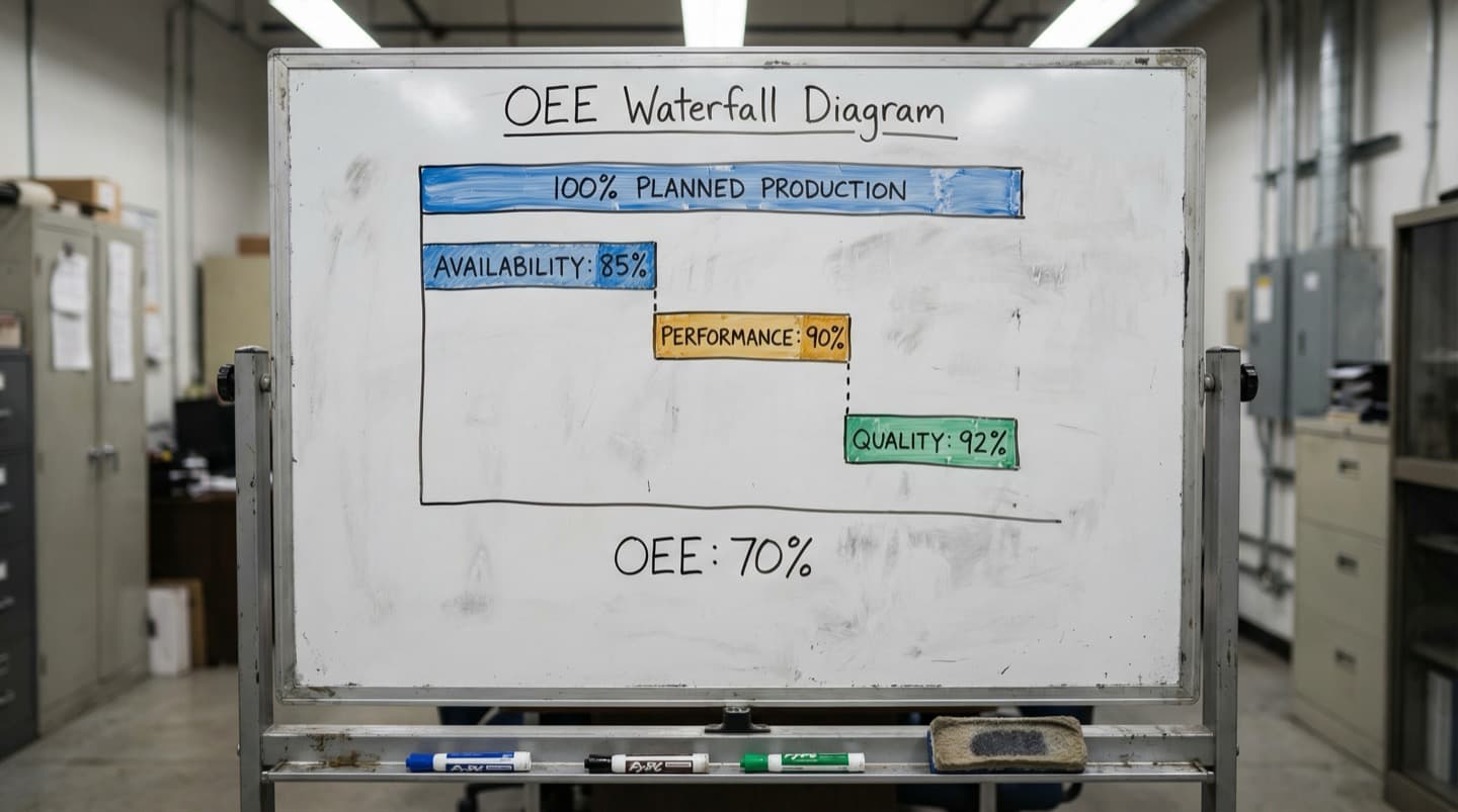
OEE multiplies three percentages: availability (uptime vs. planned production time), performance (actual speed vs. rated speed), and quality (good parts vs. total parts). A plant running 90% availability, 95% performance, and 99% quality scores 84.6% OEE. World-class OEE for discrete manufacturing is 85% [1]. The global median sits closer to 60%.
OEE is the most commonly cited manufacturing metric, and the most commonly misunderstood. The formula itself is simple: Availability x Performance x Quality. But the definitions of each component determine whether your OEE number is useful or misleading.
Availability = Run Time / Planned Production Time. Planned production time excludes scheduled breaks, planned maintenance, and periods when the line isn't scheduled to run. The key question is whether you're counting changeover time as an availability loss (you should) and whether you're counting minor stops under 5 minutes (many plants don't, which inflates the number).
Performance = (Total Parts / Run Time) / Ideal Cycle Time. This is where hidden losses live. If a machine is rated for 120 parts per minute but you're running it at 105 because "that's where it runs best," you're carrying a 12.5% performance loss that most plants never question. The rated speed should be the nameplate speed or the best demonstrated speed, not the current operating speed.
Quality = Good Parts / Total Parts. This includes startup scrap, in-process defects, and anything that doesn't meet spec on the first pass. Reworked parts that eventually pass should still count against quality because they consumed capacity without producing sellable output.
The multiplication effect is why OEE is so hard to improve. If each component is at 90%, OEE is 72.9%, not 90%. Small losses in each category compound. A 3% improvement in availability, a 2% improvement in performance, and a 1% improvement in quality might not sound like much individually, but combined they can move OEE by 5-6 percentage points, which translates to significant additional production capacity.
The first step to improving OEE is getting the measurement right. If your OEE is above 90%, either you have a world-class operation or your definitions are too generous. Most plants that claim 90%+ OEE are excluding losses that should be counted [2].
2. Availability: Finding Hidden Downtime
Availability is the component most plants measure first, but hidden downtime inflates the number. Short stops under 5 minutes, excessive changeover time, and equipment warm-up periods are often excluded from availability calculations. Including them typically drops the real availability by 5-12 percentage points.
Start by auditing what your availability calculation actually includes. Pull the last month of production data and compare total scheduled time against the downtime your system recorded. If the gap is less than 2%, your tracking is either excellent or your system isn't catching short stops.
The most common hidden downtime sources:
Minor stops (under 5 minutes): a jam that the operator clears in 90 seconds, a sensor fault that triggers a reset cycle, a material feed issue that pauses the machine briefly. Individually these are insignificant. Collectively they often add up to 30-90 minutes per shift. Many production tracking systems only log stops over 5 minutes, so this time disappears from the data.
To capture minor stops, use the machine's own cycle counter. If the machine is rated for 120 cycles per minute and should produce 57,600 parts in an 8-hour shift, but actually produces 51,200, there are 6,400 lost cycles somewhere. After accounting for quality rejects and recorded downtime, the remainder is your minor stop and speed loss bucket.
Changeover time: this is a legitimate availability loss, but many plants accept current changeover durations as fixed. A basic SMED (Single-Minute Exchange of Die) analysis on your longest changeover often reveals that 30-40% of the changeover time consists of tasks that could be done while the machine is still running the previous job (staging tools, preparing materials, pre-heating).
Start-up and warm-up time: machines that need 15-30 minutes to reach stable operating temperature after a break or shift start are losing availability. The loss is especially significant if it happens at every shift change. Some plants run machines through a warm-up cycle at the end of a break rather than the beginning, so the machine is ready when the operator returns.
For each hidden downtime source, quantify the total minutes lost per week. Focus improvement efforts on the category that's largest. Most plants find that minor stops or excessive changeover time accounts for 40-60% of their total availability gap.
3. Performance: The Speed Loss Nobody Tracks
Performance losses are the most overlooked OEE component because the machine is technically running. It's just running slower than its rated speed. Rate reductions to avoid quality issues, speed settings that were lowered for a test and never restored, and cycle time drift from worn tooling collectively cost most plants 8-15% of their theoretical output.
Ask any machine operator: are you running at rated speed? The honest answer in most plants is no. And the reasons are usually practical: running at full speed causes more jams, produces more scrap, or wears tooling faster. The operator found a speed that "works" and nobody questioned it.
The problem is that a 10% speed reduction across an 8-hour shift is 48 minutes of lost capacity. Multiply that across 5 lines and 250 production days, and the plant is giving up the equivalent of 25 production days per year without anyone tracking it as a loss.
Common sources of performance loss:
- Chronic rate reduction: the machine was slowed down 6 months ago because of a quality issue. The quality issue was fixed, but nobody restored the speed. This happens more often than anyone admits. Walk the floor and compare actual cycle times against the rated cycle times in your production system. Discrepancies of 5-15% are common.
- Speed variation within a run: the machine starts at rated speed, but the operator slows it down periodically to "let it catch up" or prevent a known intermittent issue. These micro-slowdowns don't register as stops but reduce average throughput by 3-8%.
- Idling and minor stops: the machine is powered on and in cycle, but waiting for material, waiting for downstream equipment to clear, or running empty because the infeed is starved. These are not availability losses because the machine isn't technically down. They're performance losses because the machine is cycling without producing output.
- Tooling wear: as cutting tools, forming dies, or sealing bars wear, cycle time increases to maintain quality. A fresh tool might run at 100% speed. The same tool at 80% of its life might be running at 92% speed. If tools are changed on a calendar rather than on condition, the tail end of the tool life drags down average performance.
The fix starts with transparency. Display the actual vs. rated speed on the HMI or production board for every machine. When the gap is visible, the conversation about why it exists happens naturally [3].
4. Quality: Catching Defects at the Source
Quality losses hit OEE twice: once directly through the quality factor, and once indirectly because scrap and rework consume machine capacity that could have produced good parts. A 2% quality loss doesn't just reduce OEE by 2 points; it also reduces effective availability because the machine was occupied making parts that went into the scrap bin.
Most quality losses follow a pattern: they cluster around specific conditions. The first 15 minutes after startup. The period right after a changeover. A specific material lot. A particular shift. The afternoon hours when the building warms up.
To improve the quality component of OEE, stop tracking defects by type and start tracking them by condition. When defects are sorted by type (surface finish, dimensional, contamination), the corrective actions tend to be generic: retrain operators, tighten specifications, add inspection. When defects are sorted by the conditions under which they occurred, the corrective actions become specific and actionable.
Build a matrix of defect rate against operating conditions:
- Defect rate by time since startup (first 30 minutes vs. steady state)
- Defect rate by time since changeover
- Defect rate by material lot number
- Defect rate by shift
- Defect rate by ambient temperature band (if you're monitoring it)
- Defect rate by tool wear count
This matrix almost always reveals that 60-70% of defects occur under a small set of specific conditions [4]. Fixing the conditions fixes the defects.
For startup scrap, the fix is often a standardized startup sequence with defined parameter ramp rates. For changeover-related quality loss, it's a first-article inspection protocol with defined acceptance criteria before running at full speed. For material-related defects, it's correlating incoming material properties with machine parameters.
One pattern that gets overlooked: quality losses caused by upstream equipment. The forming machine produces a part that's within spec, but at the edge of the tolerance band. The downstream assembly machine handles the nominal dimension fine, but the off-center part causes a jam or a fit issue. Each machine's quality data looks acceptable in isolation. The system-level quality problem only becomes visible when you track parts through the complete process.
5. Putting It Together with Spatial Data
The three OEE components interact with each other and with the physical environment in ways that time-series data alone can't reveal. Mapping availability losses, performance gaps, and quality events onto the floor plan shows where problems cluster, how they propagate between machines, and which environmental factors contribute.
OEE data is typically viewed per-machine or per-line as a time-series chart. Machine 4 ran at 72% OEE yesterday. The trend over 30 days is flat. That's useful but incomplete.
What's missing is spatial context. Machine 4's OEE dropped because performance fell to 88% in the afternoon. The time-series chart shows the drop. It doesn't show that machines 3, 4, and 5 all experienced performance drops between 1 PM and 3 PM, that they're all in the south-facing bay of the building, and that ambient temperature in that bay exceeds 30 degrees C every afternoon in summer.
Spatial OEE analysis overlays availability, performance, and quality metrics onto the physical floor plan. This view answers questions that per-machine analysis cannot:
- Are availability losses clustered in one area? (Points to shared infrastructure: power, utilities, environmental conditions)
- Do performance losses correlate with physical proximity? (Points to upstream/downstream dependencies or environmental factors)
- Do quality losses on one machine correlate with the output variation of the preceding machine? (Points to process interaction effects)
The practical approach is straightforward. Export your OEE data with machine location coordinates. Color-code each machine on the floor plan: green for above target OEE, yellow for within 10% of target, red for below. Update daily. Within a week, spatial patterns become visible.
Plants that adopt spatial OEE views commonly find that 20-30% of their total OEE losses are driven by environmental or infrastructure factors that are invisible in per-machine analysis. Fixing an HVAC zone, rebalancing an electrical feeder, or addressing a shared compressed air pressure drop can improve OEE across multiple machines simultaneously.
The compounding effect is significant. If a single environmental fix improves performance on 5 machines by 3% each, the aggregate capacity gain is equivalent to improving one machine by 15% but much easier to achieve because you're addressing one root cause instead of five separate symptoms.
Spatial OEE: The Dimension Most Plants Miss
Some manufacturing teams now use digital twin platforms to add a spatial dimension to OEE analysis. By mapping every OEE component onto a floor plan model, they see patterns across machines, across lines, and across environmental zones that per-machine dashboards completely miss.
The standard OEE improvement methodology goes like this: measure per-machine, identify the biggest loss category, fix the specific cause, repeat. This works well for individual machine issues. It fails for systemic issues that span multiple machines or stem from environmental factors.
Digital twin platforms address this gap by providing a spatial framework for OEE data. Each machine's availability, performance, and quality metrics are rendered on a model of the production floor. Instead of scrolling through tables of numbers, the operations team sees a heat map: areas of the plant where OEE is healthy, and areas where it's degraded.
The spatial view is especially powerful for identifying performance losses. When five machines in the same bay all show 5-8% performance degradation during the same hours, the spatial view makes the cluster obvious. The cause is usually shared: ambient temperature, vibration from a nearby process, or a utility supply issue. The per-machine view treats each as an independent problem and either never connects them or takes months to do so.
Quality losses benefit from spatial analysis too. When first-pass yield drops on a downstream machine, the spatial view lets you quickly check whether upstream machines in the same production flow had any parameter shifts. Following the physical flow path through the floor plan is more intuitive than cross-referencing time-stamped data from separate machine databases.
The maturity progression for most plants follows a predictable path: start with basic OEE tracking per machine, then add shift-level and time-based breakdown, then overlay the data onto a spatial floor plan. Each step reveals a category of losses that the previous view hid. Plants that reach the spatial analysis stage report finding an additional 8-15% of hidden losses that were invisible in per-machine or per-line views.
FAQ
Frequently Asked Questions
Related Resources
Manufacturing Downtime Cost Calculator
Calculate the true cost of unplanned downtime across your production lines. Includes lost revenue, labor waste, and scrap costs. Free, instant results.
Learn moreDigital Twin vs SCADA
A practical comparison of SCADA and digital twin platforms for manufacturing. Covers data models, visualization, alerting, and deployment trade-offs.
Learn moreDigital Twin vs MES
A practical comparison of MES and digital twin platforms for manufacturing. Covers ISA-95 levels, OEE tracking, production traceability, and how the two systems complement each other.
Learn moreDigital Twin vs Dashboards
How industrial dashboards and digital twins compare on data visualization, troubleshooting, and cross-system monitoring. Covers Grafana, Power BI, and spatial alternatives.
Learn moreUnplanned Downtime Prevention
Most manufacturers discover downtime after it costs them. Sandhed gives you the visibility to catch equipment issues before they shut down production.
Learn moreMaintenance Management
Maintenance teams lose hours tracking down service records, chasing overdue tasks, and figuring out what was done last time. Sandhed puts every work order, service record, and maintenance schedule on your 3D floor plan where you can see it.
Learn moreHow to Reduce Equipment Downtime: 8 Strategies Ranked by Impact
Reducing equipment downtime starts with knowing where you're losing time, not with buying technology. The eight strategies below are ranked by how much downtime they typically eliminate in the first year. The top three are organizational fixes that cost almost nothing. The rest require incremental investment but build on each other.
Learn moreHow to Monitor a Factory Floor in Real Time
Real-time factory monitoring means having sensor data from machines, environment, and process parameters available within seconds, not hours. It starts with choosing the right sensors for your top failure modes, runs through an edge-to-cloud architecture that handles the data volume, and works only if the alert design respects your operators' attention.
Learn moreSources
- Seiichi Nakajima / Japan Institute of Plant Maintenance — Introduction to TPM: OEE World-Class Benchmarks
- LNS Research — 2023 Manufacturing Operations Survey: OEE Measurement Practices
- IndustryWeek — Speed Losses in Manufacturing: The Hidden OEE Killer
- American Society for Quality (ASQ) — Defect Clustering and Condition-Based Quality Analysis
- McKinsey & Company — Digital Manufacturing: Unlocking Hidden Factory Capacity
See Where Your OEE Losses Actually Live
Map availability, performance, and quality data onto your floor plan and spot the spatial patterns that per-machine reports miss.